User’s Guide for SurveyingCalculation plugin for QGIS 2.x

The SurveyingCalculation plugin was created by the DigiKom Ltd (Hungary). It was supported by the SMOLE II for Niras Finland Oy. It was developed for the Land Parcel Cadastre of Zanzibar.

Hardware and software requirements

The SurveyingCalculation plug-in can be used on any computer on which QGIS 2.x can run. It was tested on Windows 7 and Fedora Linux, but it should work on other Windows versions or Linux distros . QGIS version 2.2, 2.4 and 2.6 were used for testing the plugin.

The network adjustment and the free station calculation in the plug-in is based on the GNU Gama open source project. GNU Gama must be installed separately to use these calculations.

Installation of the SurveyingCalculation plugin

Installing from QGIS Plug-in repo

1. Start QGIS
2. In the plug-in dialog enable experimental plugins (after evaluating the plugin by the QGIS community it will be changed to standard (non experimental) plugin)
3. Look for SurveyingCalculation plug-in in the list of All or Not installed list and press Install button

Installing from GitHub

If you have a Git client on your machine (Git Bash or other clients):

1. git clone the plug-in from https://github.com/zsiki/ls to ~/.qgis2/python/plugins/SurveyingCalculation on your local machine (~ is your home directory on Linux, replace it on Windows)
2. Open the QGIS Desktop

If you don’t have a Git client:

1. Download the ZIP file from https://github.com/zsiki/ls/archive/master.zip to your computer
2. Unzip it to ~/.qgis2/python/plugins/SurveyingCalculation
3. Open the QGIS Desktop

After installing the plug-in you must enable it in the Manage and Install Plugins dialog. Then the menu and the toolbar of the plug-in will be visible.

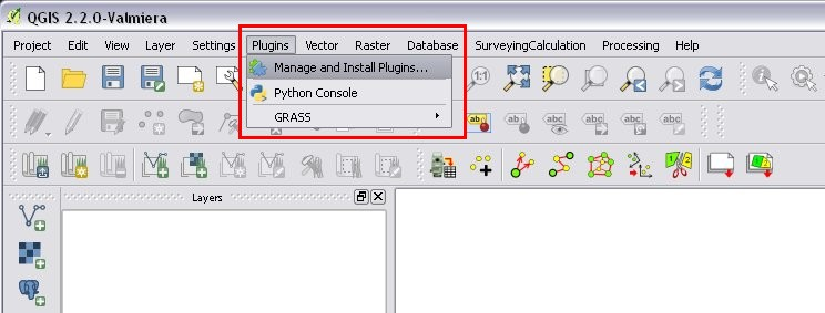
(1.) Manage and Install Plugins

Is the SurveyingCalculation plugin switched on?

(2.) Installed SurveyingCalculation plug-in

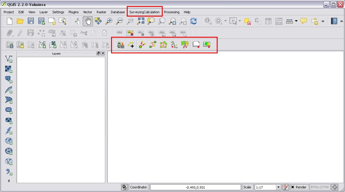
(3.) SurveyingCalculation plugin in QGIS (menu and toolbar)

GNU Gama project: gama-local

Beside installing the plug-in you also have to install gama-local (part of the GNU Gama project) for free station and adjustment calculations. See: https://www.gnu.org/software/gama

Settings before use

Settings described in this section are optional.

Check and change the settings in the config.py file. The following variables can be set in the config:

fontname:monospace font used in the calculation results widgets on Linux, the default courier font doesn’t exists on most Linux boxes fontsize:font size used in the calculation results widgets on Linux homedir:starting directory used for loading fieldbooks from log_path:full path to log file, the program must have write access right to the directory and the file line_tolerance:snapping to vertex tolerance used by line tool area_tolerance:area tolerance for area division, if the difference between the actual area and the requested area is smaller than this value, the iteration is stopped max_iteration:maximal number of iterations for area division

If you change any value in the config.py file, the QGIS plug-in have to be reloaded or QGIS must be restarted.

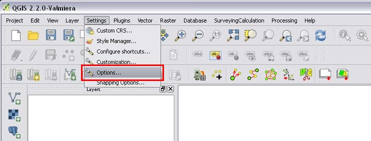
Set the default coordinate reference system (CRS) for new projects and new layers on the CRS tab in the Setting/Options menu to the local CRS.

Set the Representation for NULL values to empty string on the Data sources tab in the Setting/Options menu. It makes the Attribute Table (Fieldbook) more readable.

(4.) Settings of Attribute Table

(5.) Settings of Attribute Table

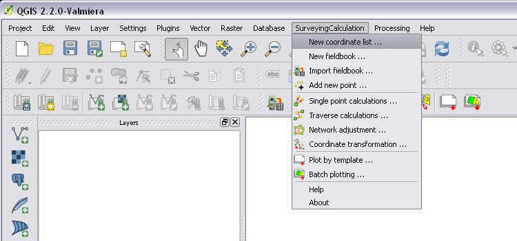
Most of the cases you need an open coordinate list to store calculation results. Open an existing QGIS project which contains a coordinate list (a point shape file whose name have to start with coord_) or create a new project and add an existing coordinate list to the project by the add vector layer icon or create a new project and create a new coordinate list from the SurveyingCalculation/New coordinate list ... menu.

Check the coordinate reference system (CRS) of your coordinate list (Properties from the popup menu of the layer) and the map.

After loading an existing one or creating a new Coordinate list shape file, you get a point layer in your project with the following columns in the attribute table (column names and types are mandatory):

point_id:point number (string 20) e:East coordinate (number 12.3) n:North coordinate (number 12.3) z:Z coordinate (elevation) (number 8.3) pc:point code (string 20) pt:point type (string 20)

The first three columns (point_id, e and n) are obligatory, you have to fill them. You mustn’t rename or erase these columns but you can add new columns to the attribute table.

You can edit the coordinate list if you push Toggle Editing Mode for this layer. Be careful:

do not edit the coordinates manually, because the point position won't change automatically
do not add new point by mouse click, because the coordinate columns in the table won't change automatically

Use the Add new point dialog to update coordinates and location together.

(6.) New coordinate list

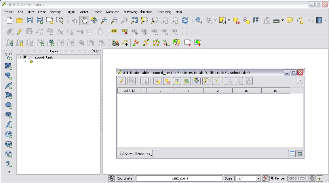
(7.) Empty coordinate table

Only one coordinate list should be open in a project at a time.

Importing fieldbooks

Observations made by total stations and GPS are stored in electric fieldbooks. The files storing the fieldbook data have to be downloaded to the computer before you can use them in the plug-in. Different fieldbook types are supported:

• Leica GSI 8/16
• Geodimeter JOB/ARE
• Sokkia CRD
• SurvCE RW5
• STONEX DAT

Any number of electric fieldbooks can be opened/loaded into a QGIS project. You can even create a new empty fieldbook and fill it manually.

1. There must be an open coordinate list in your actual project (a point layer whose name starts with coord_). Otherwise coordinates read from the filedbook will be lost

2. Click on the Load fieldbook icon or select it from the SurveyingCalculation menu

3. Choose the type of the fieldbook (Geodimeter JOB/ARE; Leica GSI; Sokkia CRD, SurvCE RW5, STONEX DAT)

4. Select the output DBF file where your observations will be stored, the name will start with fb_, the program will add it to the name automatically if you forget it

5. After giving the path to the DBF file the new fieldbook will be added to your QGIS project. The name of the fieldbook always starts with “fb_”. This database table stores measurements only, it has no graphical (map) data. Fields in the table:

   id:ordinal number of observation in fieldbook, sort by this field normally point_id:point number (max 20 characters) station:if record data belongs to a station it must be station otherwise empty hz:horizontal angle or orientation angle in station record v:zenith angle sd:slope distance (horizontal distance if zenith angle is empty) th:target height or instrument height in station record pc:point code

You musn’t change the name of columns or erase them, but you can add new columns to the table.

The loader adds an extra column to the observation data, the id column, sorting the table by this column gives the right order of the observations.

You can create an empty fieldbook for manual input using the New fieldbook from the SurveyingCalculation menu.

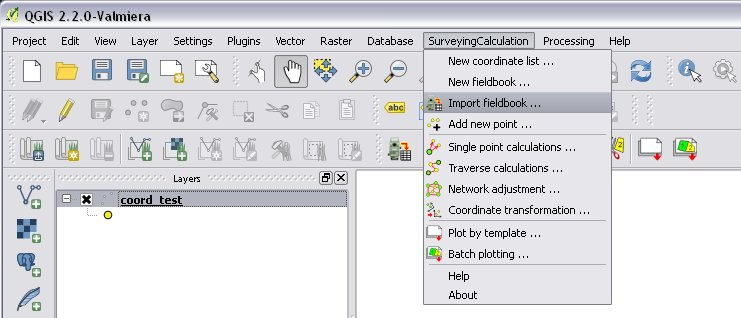
(8.) Import fieldbook menu

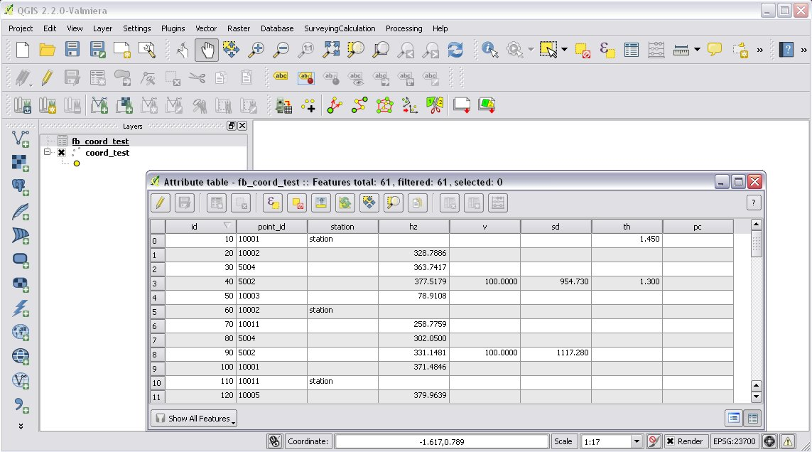
(9.) Fieldbook attribute window

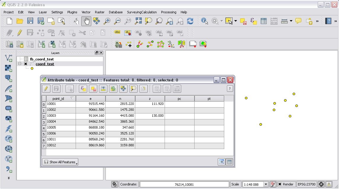
(10.) Coordinate list

Leica GSI

Both the 8 byte and 16 byte GSI files are supported. As there are no standard markers for station start in GSI files, you can use code block to mark a new station in observations or you have to have a record with station coordinates or instrument height to mark the start of a new station.

Code block to mark the start of a station:

410001+00000002 42....+12012502 43....+00001430

410001+00000002

Code 2, start of a new station

42....+12012502

Station id is 12012502

43....+00001430

Instument height 1.430 m (optional)

Data codes handled, loaded from GSI:

11:point id 21:horizontal angle (hz) 22:vertical angle (v) 31:slope distance (sd) 41:code block 42:station id 43:station height 71:point code (pc) 81:easting 82:northing 83:elevation 84:easting of station 85:northing of station 86:elevation of station 87:target height (th) 88:station height (overwrites 43 code)

The different units in the electric fieldbook are converted to GON and meters during the import.

Geodimeter JOB/ARE

JOB and ARE are separate data files. Observations and optional coordinates are stored in JOB file. Only coordinates are stored in ARE file. After loading a .JOB you can optionally load an .ARE file in the same way.

Data codes handled, loaded from JOB/ARE:

2:station id 3:instrument height 4:point code (pc) 5:point id 6:target height (th) 7:horizontal angle (hz) 8:zenith angle (v) 9:slope distance (sd) 23:units 37:northing 38:easting 39:elevation 62:orientation point id

The different units in the electric fieldbook are converted into GON and meters during the import.

Sokkia CRD

Sokkia CRD loader can handle two softly different file format SDR33 and SDR20.

Data records handled, loaded from CRD:

00:header record 02:station record 03:target height 08:coordinates 09:observations

The different units in the electric fieldbook are converted into GON and meters during the import.

SurvCE RW5

The SurvCE program RW5 format can store total station and GPS observations. Both type of data can be loaded into QGIS.

Data records handled, loaded from CRD:

GPS:latitude, longitude from GPS receiver –GS/SP:projected coordinates (overwrites latitude, longitude) OC:station record TR/SS/BD/BR/FD/FR:  observation record BK:orientation record LS:instrument height and target height record MO:units record

The different units in the electric fieldbook are converted into GON and meters during the import.

STONEX DAT

Unfortunately we had no description for this fieldbook format, we reverse engineered information from the sample file we got. GON angle units and meters are supposed for the data in the DAT file.

Data records handled, loaded from DAT:

K:station and orientation angle E:observation record B/C:coordinate record L:orientation direction record

Using fieldbook data

Angles are displayed in the fieldbook in Grads (Gon) units with four decimals. Distances, instrument and target heights are in meters.

Sort the fieldbook by the id column, to have the right order of observations.

Data in the loaded fieldbooks can be changed, records can be inserted, updated and deleted. You can use the standard QGIS tools to change or extend fieldbook data. Open the fieldbook Attribute Table, turn on Toggle Editing Mode.

Insert record: Click on the Add feature button and fill in the record. Use the right id (first column) for the row to get the right position in the fieldbook.

Delete record: Select the records to be deleted and click on the Delete selected features button.

Update record: Double click on the field you want to change and edit the data.

After editing the fieldbook data you have to save the changes, click the Save Edits or Toggle Editing Mode button.

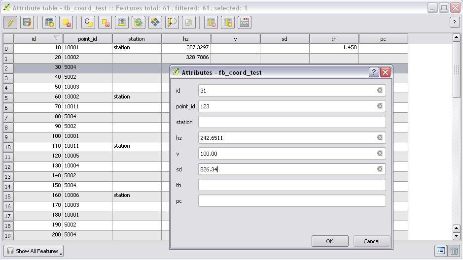
(11.) Add feature to Fieldbook

Add new point to the Coordinate list

In the Add new point dialog you can manually add new points to the coordinate list. The Add new point dialog can be opened from the SurveyingCalculation menu. The Point ID, East, North fields must be filled, the others are optional. Use the Add button to add the point to the coordinate list. The Add button saves the new point and resets the form. The Close button closes the dialog window.

This dialog can be used to overwrite existing coordinates in the coordinate list, too. If you input an existing point, a warning will be displayed and you can decide whether to continue to store point.

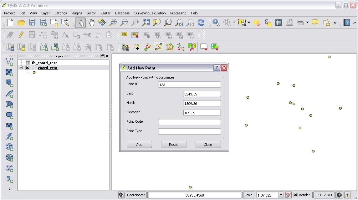
(12.) Add new point to the Coordinate list

You can use the standard QGIS Add Delimited Text Layer button to bulk import coordinates from CSV or TXT files. The restrictions are

• the column names must be the same as discribed before (point_id, e, n, z, pc, pt)
• the column types must be the same as discribed before, a CSVT file can be created to define column types, the name of the CSVT file have to be the same as the CSV file
• the name of result shape file have to start with coord_

Sample CSVT file to load coordinate lists:

String(20),Real(12.3),Real(12.3),Real(8.3),String(20),String(20)

Single Point Calculations

During the calculations the plug-in will use the data from the opened fieldbooks (fb_ tables) and from the opened coordinate list (coord_ layer).

In the single calculation dialog you can calculate coordinates of single points using trigonometric formulas.

All calculations can be repeated, the last calculated values will be stored, the previous values are lost.

A SurveyingCalculation plug-in maintains a log file, a simple text file. The details of calculations are written to the log. The location of the log file can be set in the config.py.

In the different lists of the dialog you can see the fieldbook name and the id beside the point name. These are neccessary to distinguis stations if the same station was occupied more then once, or directions if the same direction was measured from the same station more than once.

Orientation

Orientation of stations is neccessary to solve intersection, radial survey and some type of traversing line. During the orientation no coordinates are calculated.

To calculate orientation angle on a station do the following:

1. Click on the Single Point Calculations icon to open the Single Point Calculation dialog.
2. Select the Orientation from the Calculation group.
3. Select the station id from the Station (1) list. You can calculate the orientation of one station at a time.
4. The Target Points list is filled automatically, with the directions to known points from the selected station.
5. Add to Used Points list one or more points which you would like to use for the orientation. If you would like to change the Used Points list, use the Remove button.
6. Click on the Calculate button.
7. Results of calculation are displayed automatically in result widget and sent to the log file.
8. You can change settings in the dialog and press Calculate to make another calculation, use the Reset button to reset the dialog to its original state.

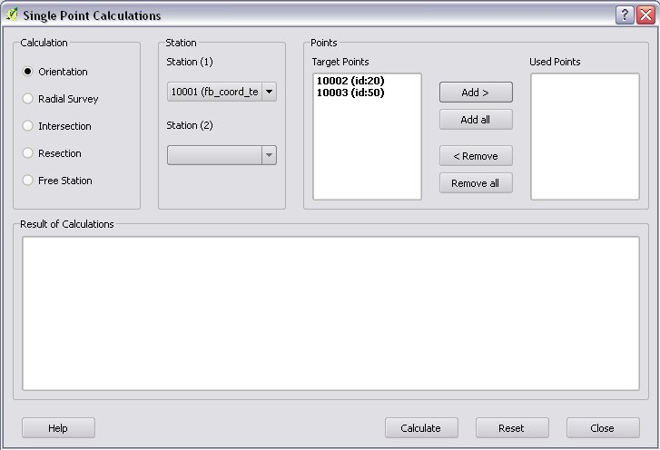
(14.) Orientation

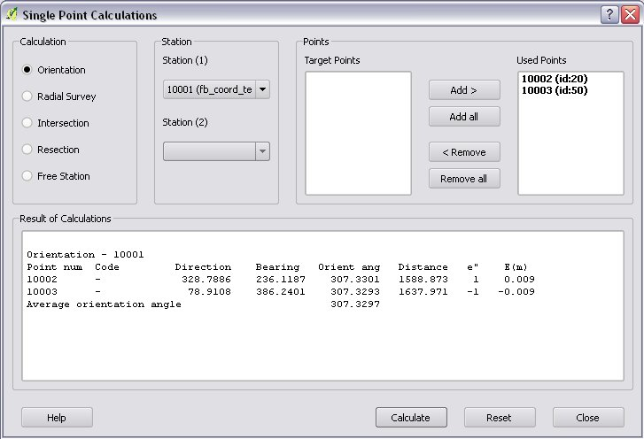
(15.) Result of Orientation

Radial Survey (Polar Point)

Beside the horizontal coordinates the elevation is also calculated for polar points if the instrument height, the target height and the station elevation are given.

1. Click on the Single Point Calculations icon to open the Single Point Calculations dialog
2. Select Radial Survey from the Calculation group.
3. Select the Station id from the Station (1) list. The list contains only points with orientation angle. You can calculate several polar points from the same station at a time.
4. The Target Points list is filled automatically with the points observed from the selected station. The points in bold face have coordinates.
5. Add one or more points to the Used Points list, which you would like to calculate coordinates for. If you would like to change the Used Points list, use the Remove button.
6. Click on the Calculate button.
7. Results of calculation are displayed automatically in result widget and sent to the log file.
8. You can change settings in the dialog and press Calculate to make another calculation, use the Reset button to reset the dialog to its original state.

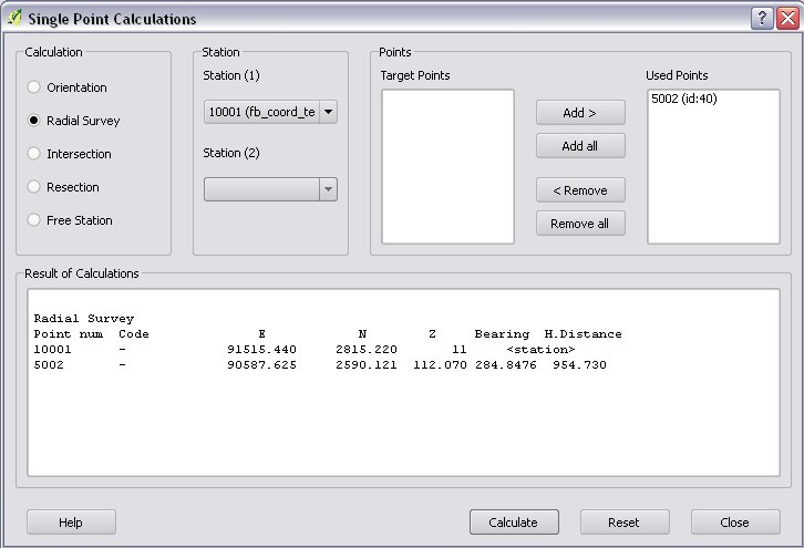
(16.) Radial Survey

Intersection

You can calculate horizontal coordinates for one or more points, which directions were observed from two known stations.

Before the intersection calculation the used stations must be oriented.

To calculate intersection do the following:

1. Click on the Single Point Calculations icon in the toolbar to open the Single Point Calculations dialog.
2. Select Intersection from the Calculation group.
3. Select two known stations from the Station(1) and Station(2) lists. The lists contain only points with orientation angle.
4. The Target Points list is filled automatically. It contains the points measured from both stations. The points in bold face have coordinates.
5. Add one or more points to the Used Points list which you would like to calculate coordinates for. If you would like to change the Used Points list, use the Remove button.
6. Click on the Calculate button.
7. Results of Calculation are displayed automatically in result widget and sent to the log file.
8. You can change settings in the dialog and press Calculate to make another calculation, use the Reset button to reset the dialog to its original state.

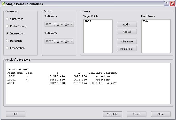
(17.) Intersection

Resection

You can calculate horizontal coordinates of a station if at least three known points were observed from there.

To calculate resection do the followings

1. Click on the Single Point Calculations icon in the toolbar to open the Single Point Calculations dialog.
2. Select Resection from the Calculation group.
3. Select the station id from the Station (1) list. The list contains all stations. The stations in bold face have coordinates.
4. The Target Points list is filled automatically. The list contains the known points, which were measured from the station. You can calculate the coordinates of one station at a time.
5. Add exactly three points to the Used Points list which will be used for resection. If you would like to correct, use the Remove button.
6. Click on the Calculate button.
7. Results of calculation are displayed automatically in result widget and sent to the log file.
8. You can change settings in the dialog and press Calculate button to make another calculation, use the Reset button to reset the dialog to its original state.

(18.) Resection

Free Station

You can calculate the horizontal coordinates of a station from directions and distances using the least squares method.

To calculate free station do the following:

1. Click on the Single Point Calculations icon in the toolbar to open the Single Point Calculations dialog.
2. Select Free Station from the Calculation group.
3. Select station id from the Station (1) list. The list contains all stations. The stations in bold face have coordinates.
4. The Target Points list is filled automatically. The list contains the known points, which were measured from the selected station. You can calculate the coordinates of one station at a time.
5. Add two or more points to the Used Points list which will be used for calculation. If you would like to correct, use the Remove button.
6. Click on the Calculate button.
7. Results of calculation are displayed automatically in the result widget and sent to the log file.
8. You can change settings in the dialog and press Calculate to make another calculation, use the Reset button to reset the dialog to its original state.

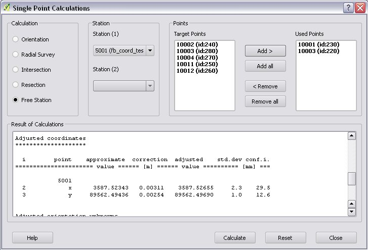
(19.) Free Station - Adjusted coordinates

The result list of the adjustment is very long. Consult the GNU Gama documentation for further details.

Free station calculation uses the default standard deviations (3cc, 3mm+3ppm) for the adjustment.

Traverse Calculations

During the traverse calculations the plug-in will use the data from the opened fieldbooks (fb_ tables) and from the opened coordinate list (coord_ layer).

It is possible to calculate three different types of traverse.

1. Closed traverse: Closed (polygonal or loop) traverse starts and finishes at the same known point. This point must be oriented.
2. Link traverse: A closed link traverse joins two different known points. None, one or both ends can be oriented.
3. Open traverse: An open (free) traverse starts at a known point with orientation and finishes at an unknown point.

To calculate traverse do the following:

1. Click on the Traverse Calculations icon in the toolbar to open the Traverse Calculations dialog.

2. Select the type of traverse from Type group.

3. Select the start point of traverse from the Start Point list.

4. Select the end point from the End Point list.

   • In case of closed traverse the End Point list is disabled and changes according to the Start Point list.
   • In case of link traverse the End Point list contains all known stations.
   • In case of open traverse the End Point list contains the points measured from the last point in the Order of points list. Therefore the end point should be selected after inserting and sorting all angle points in the Order of points list.

5. The Target Points list is filled automatically. The points in bold face have coordinates.

6. Add the traverse points from the Target Points list to the Order of Points list one by one.

7. The order of traverse points can be changed with Up and Down button. If you would like to correct, use the Remove button.

8. In case of open traverse select the end point now.

9. Click on the Calculate button.

10. Results of calculation are displayed automatically in result widget and sent to the log file.

11. You can change settings in the dialog and press Calculate button to make another calculation, use the Reset button to reset the dialog to its original state.

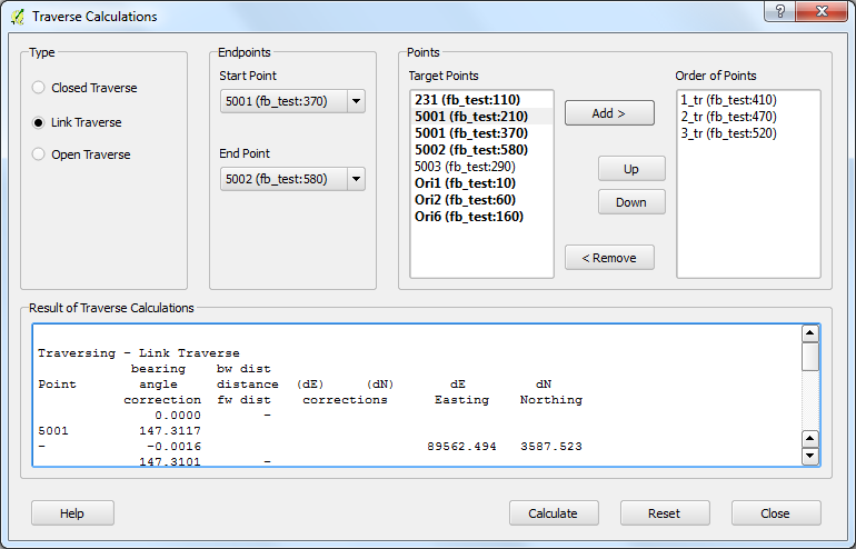
(20.) Traverse Calculation - Link traverse

In the result of calculation you can find the angle and coordinate corrections, and the coordinates of the traversing points.

Network adjustment

During the network adjusment the plug-in will use the data from the opened fieldbooks (fb_ tables) and from the opened coordinate list (coord_ layer).

Network adjustment is the best method to calculate the most probably position of observed points, when more observations were made than neccessary. By the help of GNU Gama adjustment the blunder errors can be detected, eliminated.

Free network can also be adjusted, when there are no fixed coordinates in the network. In this case some points have to have approximate coordinates.

To calculate network adjustment do the following:

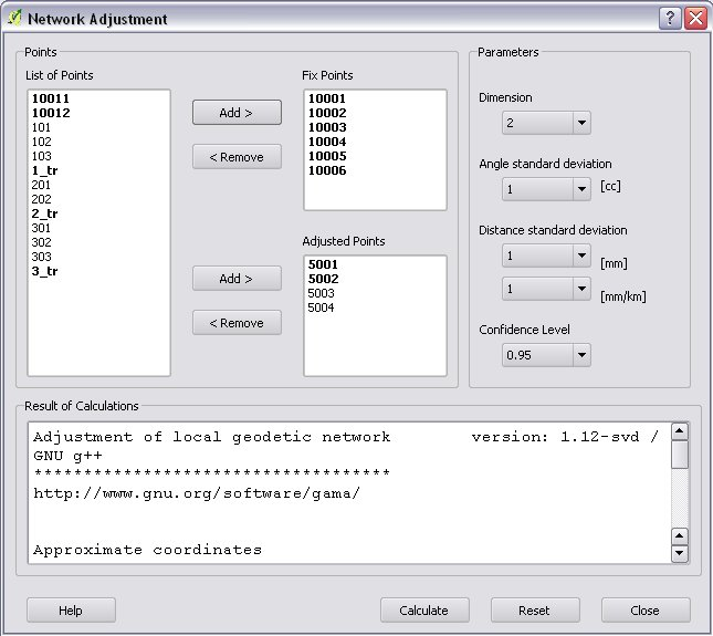
1. Click on the Network adjustment icon to open the Network Adjustment dialog.
2. Select the fix points from the List of Points and add them to the Fix points list. During the adjustment the coordinates of fix points will not be changed. Points in bold face in the List of Points have coordinates in the actual coordinate list, so only those can be added to the Fix Points list. In the List of points you can find only those points which an observation was made to.
3. Select points to adjust from the List of Points and add them to the Adjusted points list. You can add any point to the Adjusted Points.
4. Set the parameters of the adjustment. Setting the correct standard deviations are very important from the view of adjustment calculation. Set these corresponding to the used total station.
5. If you would like to correct, use the Remove button.
6. Click on the Calculate button.
7. Results of calculation are displayed automatically in result widget and sent to the log file.
8. You can change settings in the dialog and press calculate to make another calculation, use the Reset button to reset the dialog to its original state.

(21.) Network adjustment

The result list of the adjustment is very long. Consult the GNU Gama documentation for further details.

Coordinate transformation

Besides the on the fly reprojection service of QGIS, the SurveyingCalculation plug-in provides coordinate transformation based on common points having coordinates in both coordinate systems. Two separate coordinate lists have to be created with the coordinates in the two coordinate systems before starting the coordinate transformation.

The plug-in provides different types of transformation. The calculation of the transformation parameters uses the least squares estimation if you select more common points than the minimal neccessary.

Orthogonal transformation:  at least two common points Affine transformation:  at least three common points 3rd order transformation:  at least ten common points 4th order transformation:  at least fifteen common points 5th order transformation:  at least twenty-one common points

1. The coordinate list you would like to transform from has to be opened in the actual QGIS project. Do not open the coordinate list of the target system.
2. Click on the Coordinate transformation icon in the toolbar to open the Coordinate Transformation dialog.
3. The From Layer field is filled automatically with the opened coordinate list.
4. Select To Shape file where to transform to, push the button with ellipses (...) to open the file selection dialog. The transformed points will be added to this shape file.
5. The list of Common Points is filled automatically.
6. Add points from the Common Points list to the Used Points list.
7. Select the type of transformation, only those types are enabled for which enough common points were selected.
8. If you would like to correct, use the Remove button.
9. Click on the Calculate button.
10. Results of calculation are displayed automatically in result widget and sent to the log file.
11. You can change settings in the dialog and press Calculate button to make another calculation, use the Reset button to reset the dialog to its original state.

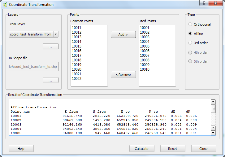
(22.) Coordinate transformation - Affine transformation

At the beginning of the result list you can find the used common points with the coordinates in both systems and the discrepancies between the target and transformed coordinates. If you find big discrepancies in the list, there are mistakes in the coordinates. At the end of the list you can find transformed points where the discrepancies are empty. These points are added to the target coordinate list.

The coordinates of those common points which were not selected for the transformation won’t be changed in the target coordinate list.

Polygon division

With the Polygon Division tool you can divide a parcel into two at a given area. There are two possible division types:

Paralel to a given line:  the line will be shifted until the right side polygon of the division line will have the given area. Through the first given point:  the line will be rotated around the first point until the right side polygon of the division line will have the given area.

1. Select the polygon layer in the layer list in which you would like to divide a polygon.
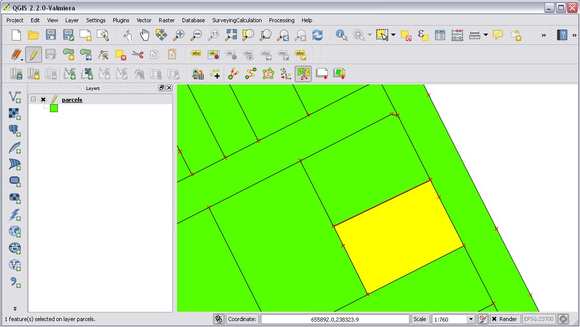
2. Select the parcel with the Select Single Feaure tool, which you want to divide.
3. Click on the Polygon Division tool in the SurveyingCalculation toolbar.
4. Click at the start point of the division line and drag the rubberband line and release the mouse button at the end point.
5. The Area Division dialog appears automatically.
6. Set the Area field and the select method. The full area field is not editable, it shows the total area of the selected polygon.
7. Set the type of division and click on the Divide button.

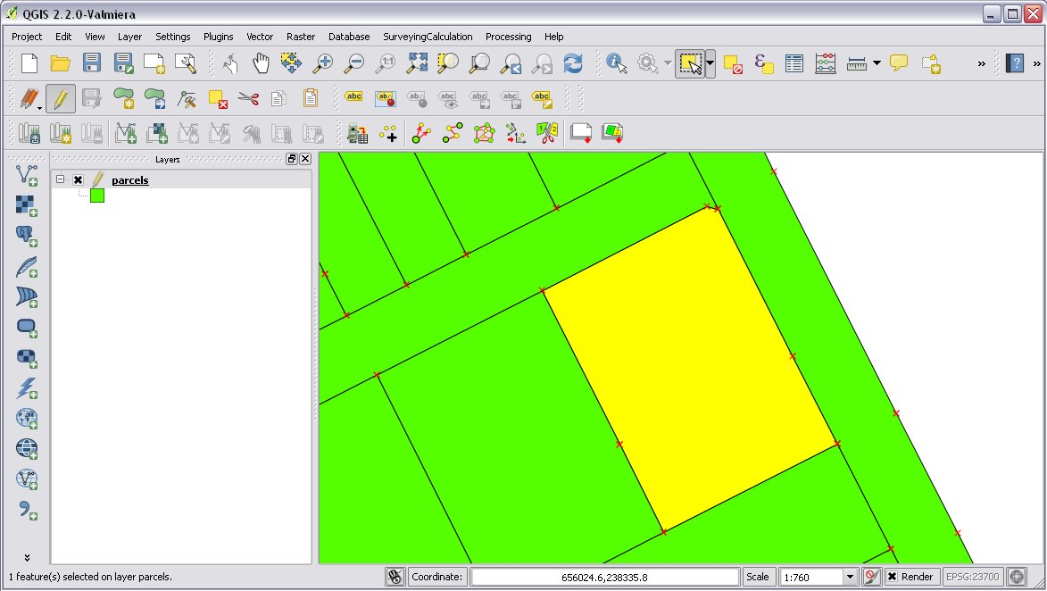
(23.) Polygon division - Selected polygon to divide

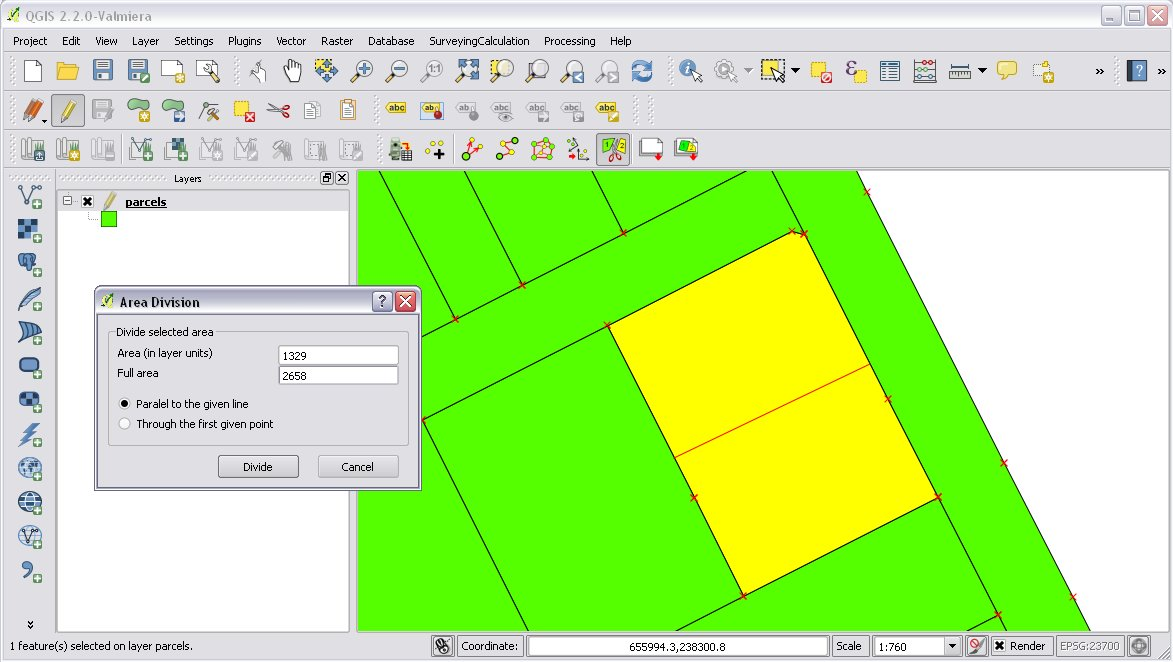
(24.) Polygon division - Area Division

(25.) Polygon division - Divided polygons

If the given divider line does not intersect the polygon border, the plug-in will extend the line. You can give a divider line outside the selected polygon, in this case only parallel division is available in the Area Division dialog.

Plot

This utility was added to the plugin for the ability to plot land parcels or other polygon type features automatically. The plugin offers two ways to achieve this:

1. Firstly you can plot the actual map view by Plot by Template command using a precreated composer template file (.qpt).
2. Secondly it is also possible to plot selected parcels (polygons) by Batch plotting command using a precreated composer template file (.qpt).

Templates can be created by the print composer of QGIS (Save as template from the menu). Look at the QGIS documentation for help.

Plot by Template

With Plot by template command you can plot the actual map view at the given scale.

1. First zoom the map view to the required area and perhaps the required scale.
2. Click on the Plot by template button in the toolbar to open the Plot by template dialog.
3. In the dialog you can select a composer template and the scale.
4. Use the Change dir... button to select a template from another directory. The default directory for templates is the template subdirectory in the plug-in installation directory.
5. In the scale list the previously set scale also appears beside some predefined scales. You can also give a new scale manually but it must be a positive integer value. The default scale is <extent> which means that the scale will be adjusted to the map view extent.
6. You can give a name to the composition optionally. If you leave blank QGIS will generate a name automatically.

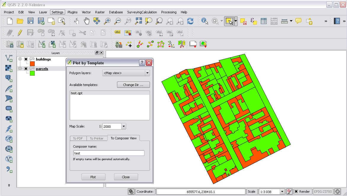
(26.) Plot by Template

In the end a composer window will appear with the map composition and it can be printed to a system printer or exported to PDF file.

Batch plotting

With the “Batch plotting” command you can plot selected polygons from one layer using a composer template file. Batch plotting creates a QGIS atlas composition, which is a multi-page composition. One polygon will be on one page. In the dialog you can choose the output of the plot.

1. This utility needs at least one polygon type layer open.
2. Select the polygons you want to plot, they must be on the same layer.
3. Click on the Batch plotting button in the toolbar to open the Batch Plotting dialog.
4. In the dialog select the layer which contains the selected polygons.
5. Select the composer template from the list. Use the Change dir... button to select a template from another directory. The default directory for templates is the template subdirectory in the plug-in installation directory.
6. From the scale list you can choose from predefined scales or give a new scale manually. It has to be a positive integer value.

There are three possible outputs of batch plot:

• export to PDF
• plot to a system printer
• open in composer view

Export to pdf

You can export the composition to a single multi-page PDF file or to separate files (individual single page PDF file for each selected polygons). In the first case give the PDF file after pressing the Plot button. In the second case you have to fill the Output filename pattern field according to the Output filename expression of QGIS. After pressing the Plot button, select the directory where you want to save the PDF files to.

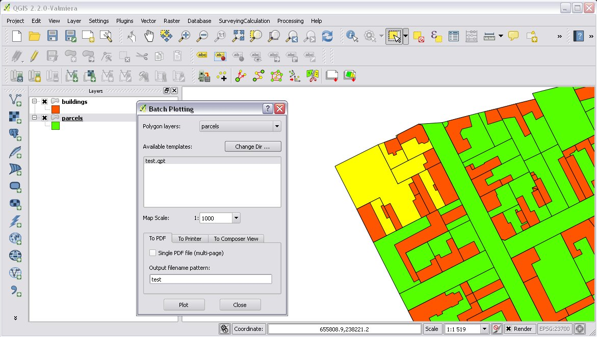
(27.) Batch plotting - Export to pdf

Plot to the system printer

It is possible to send the composition directly to the printer. After pushing the Plot button the Print settings dialog will be shown. At this point you can select the printer and the number of copies. You can’t change the other settings, because the page order is not known. Push the Print button and the composition will be printed.

Open in composer view

The third option is to view the composition in composer view. This is very similar to the Plot by template function. Since it is an atlas composition, in the composer view you can look at each page separately. Use the arrows in the toolbar to move to the previous/next page. In the Atlas generation panel the settings of the atlas composition can be modified. From the composer view you can print either a single page or all pages or export them to a PDF file.

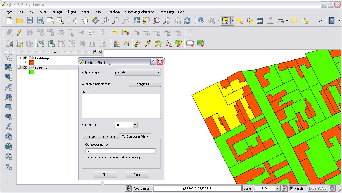
(28.) Batch plotting - Open in composer view